

You know that sim that always misses the overnight window? The one that makes your team babysit a cluster and pray the queue clears? That run just got way faster.
AWS launched Hpc8a—an AMD EC2 instance with 5th Gen AMD EPYC. It delivers up to 40% higher performance than Hpc7a, 42% more memory bandwidth, and 300 Gbps Elastic Fabric Adapter (EFA). Translation: you can chew through CFD, FEA, and weather jobs faster. You scale cleaner and likely spend less for the same or better results.
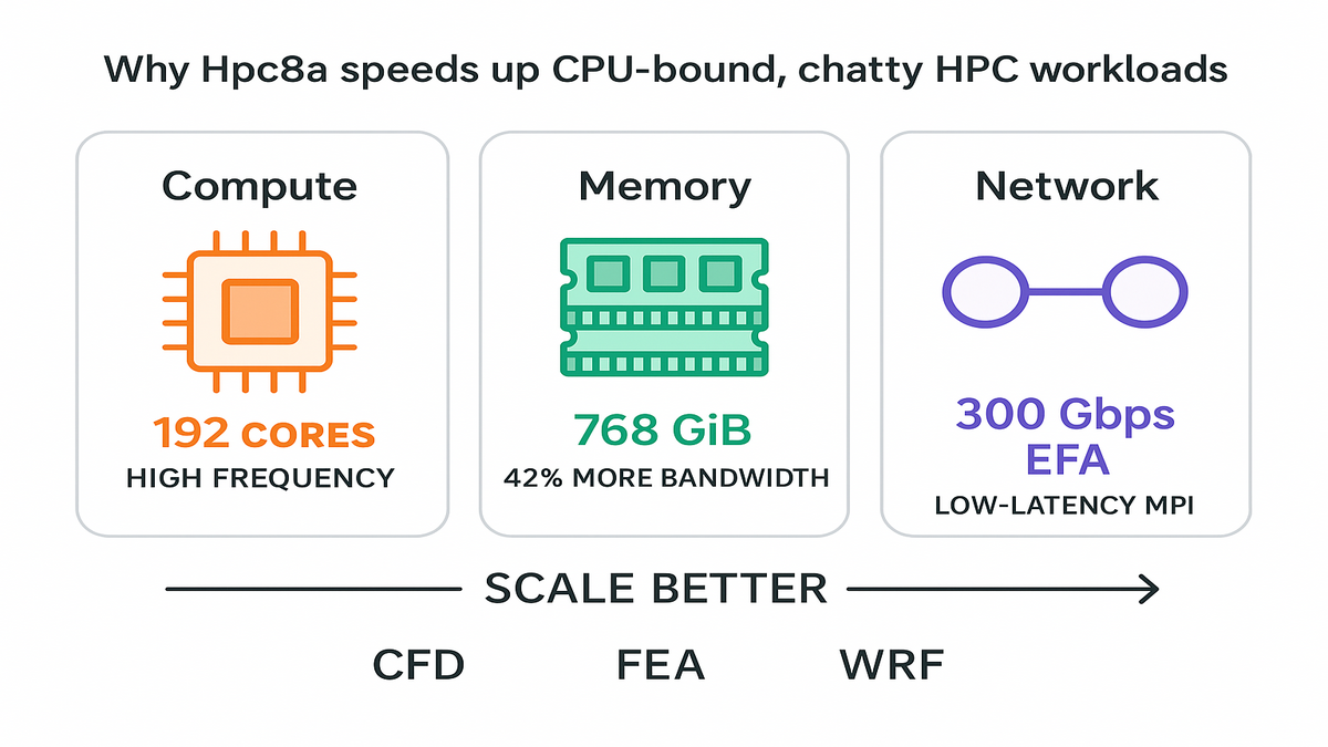
No pet projects here. We’re talking 192 high‑frequency cores and 768 GiB RAM. That’s a clean 1:4 core‑to‑memory ratio, which is nice. Plus sixth‑gen Nitro under the hood. It’s built for tightly coupled MPI jobs that punish weak interconnects. If your app chats across nodes, Hpc8a speaks fluently—and fast.
Your move? Rethink your HPC playbook. If you’ve been eyeing GPUs for everything, stop a sec. CPU‑bound math just got a real upgrade. And if your on‑prem cluster sits in procurement hell, this is your out.
TLDR
- Up to 40% faster vs. Hpc7a; 42% more memory bandwidth.
- 192 cores, 768 GiB RAM, 300 Gbps EFA for low‑latency MPI.
- Single size: hpc8a.96xlarge; EBS‑only; baseline 75 Gbps network.
- Best for tightly coupled CFD, FEA, WRF, molecular dynamics.
- Available now in US East (Ohio) and Europe (Stockholm).
- Save with Savings Plans; burst with Spot for non‑critical runs.
What Hpc8a Changes
Why this CPU jump matters
If your workload is CPU‑bound and chatty—think OpenFOAM, WRF, or explicit FEA—it’s not just flops. Your speed limit is memory bandwidth and inter‑node latency. Hpc8a lifts all three: higher‑frequency 5th Gen AMD EPYC cores, 42% more memory bandwidth vs. Hpc7a, and 300 Gbps EFA for ultra‑low‑latency MPI. That combo lets you scale without your solver face‑planting at 256+ nodes.
For you, that means fewer hacks around halo exchanges and fewer restarts. You also get a better strong‑scaling curve across more nodes. The 1:4 core‑to‑memory ratio (4 GiB per core) hits a sweet spot. Great for meshes that blow up cache but don’t need memory‑heavy SKUs.
Zooming in: strong scaling keeps problem size fixed while adding nodes. The wall time should drop when things go right. The usual failure mode is diminishing returns once communication dominates compute. Hpc8a’s extra memory bandwidth keeps per‑core kernels fed and steady. EFA’s fat pipe and low jitter keep collectives from ballooning. Think Allreduce, Alltoall, and neighbor exchanges staying tight. On real jobs—like a 30–80M cell RANS case or a 3D weather domain with tilted nesting—you avoid the cliff. You get a smooth scaling curve instead.
Also worth calling out: high clocks help the “serial islands” inside parallel codes. Geometry preprocessing, mesh partitioning, file I/O orchestration, and setup phases get faster. When those shrink, your whole pipeline flows better end‑to‑end, not just the compute kernel.
A quick mental model
- Compute: 192 high‑frequency cores keep per‑rank performance high.
- Memory: 768 GiB keeps memory‑bound kernels from starved stalls.
- Network: 300 Gbps EFA minimizes the MPI tax at scale.
First‑hand example: You run a 50M‑cell RANS CFD model across 8 nodes. On Hpc8a, you can raise ranks‑per‑node while holding memory‑per‑rank steady. Then lean on EFA to keep all‑to‑all and nearest‑neighbor exchanges tight. Net‑net: shorter wall clock without wrecking accuracy or inflating your bill.
Pro tip: Keep your ranks per NUMA domain balanced. Over‑subscribe and you’ll turn extra bandwidth into cache thrash.
Another way to picture it:
- WRF: Domain decomposition across i/j tiles loves low‑latency halos each time step. With EFA, those halos don’t stall the ensemble, so time‑to‑forecast tightens.
- Explicit FEA: The solver advances tiny time steps and needs fast global reductions. If latency is low and consistent, you push physics more and wait less.
- Molecular dynamics: Neighbor list updates and PME grids can be chatty. Faster links mean fewer long‑tail outliers per step.
Keep in mind, scaling isn’t just about adding ranks. It’s about balance. If one rank’s partition has too many boundary faces or funky geometry, it slows everything. Before you blame the network, check partition quality and reorder meshes for locality. Also verify eager and rendezvous thresholds match your usual message sizes.
Under The Hood
The silicon and system story
- 5th Gen AMD EPYC (max up to 4.5 GHz): High clocks help single‑thread‑sensitive kernels. Geometry, I/O, and decompositions speed up. Parallel sections still fly.
- Sixth‑gen AWS Nitro Cards: Offload virtualization, storage, and networking to hardware. That frees more CPU for your code and tightens tenant isolation.
- EFA at 300 Gbps: Built for HPC and ML collectives; integrates with libfabric. Your MPI stack talks to the network like it should—fast and consistent.
This isn’t a kitchen‑sink instance. AWS ships a single size—hpc8a.96xlarge. You tune via nodes and ranks, not SKU musical chairs. It’s EBS‑only, which simplifies ephemeral choices quite a bit. It also nudges you toward right‑sized FSx for Lustre scratch for hot I/O.
Under the covers, EFA uses a user‑space networking stack via libfabric. You get hardware offloads and reliable datagram transport to slash tail latency. Translation: less jitter in your collectives and more predictable iteration times. Nitro keeps noisy‑neighbor effects in check. It offloads the hypervisor and data plane, which matters if your job hates microbursts.
What that means
- MPI: Use libfabric’s EFA provider; set the right eager and rendezvous thresholds.
- I/O: Land your working set on FSx for Lustre; keep checkpoints on EBS.
- Schedulers: Use cluster placement groups; pin ranks per NUMA; set CPU affinity.
First‑hand example: A genomics pipeline has bursty I/O and shared reads. Stage reference data on FSx for Lustre for high‑throughput reads. Write checkpoints and logs to EBS for persistence. Your compute stays hot, and your storage bill stays sane.
A few tactical tips to make the hardware sing:
- MPI stacks: Confirm your provider path (e.g., libfabric/efa) is really active. Use verbose logs to verify small messages use eager and larger flip to rendezvous. If supported, test different collective algorithms for Allreduce and Alltoall. Tree vs. ring vs. recursive doubling can vary by pattern.
- NUMA awareness: Treat sockets as first‑class citizens. Map ranks to sockets and keep memory local. Bad binding turns fancy cores into glorified waiters.
- Threading: If you mix MPI + OpenMP, measure the sweet spot. Try 2–4 threads per rank instead of assuming all cores, all the time. Too many threads can fight over cache lines.
Pick Hpc8a Versus GPU Instances
CPU vs GPU tree
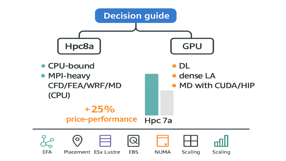
Pick Hpc8a when:
- Your solver is CPU‑bound (CFD RANS/LES, explicit FEA, WRF, molecular dynamics without heavy GPU kernels).
- You rely on MPI collectives that punish slow interconnects.
- You need predictable scaling at 100s–1000s of vCPUs without retuning CUDA.
Pick GPU instances when:
- Your code has mature GPU paths (dense linear algebra, deep learning, modern MD with CUDA/HIP backends).
- You’re memory‑bandwidth limited but can leverage HBM.
Note: amazon ec2 g3 instances (older GPU family) were great for graphics and visualization. They weren’t for state‑of‑the‑art CUDA training. If you need aws gpu accelerated instances for training or inference, use current GPU families. For long, steady workloads, aws gpu reserved instances or Savings Plans can still make sense. Hpc8a complements those well. Use CPU for meshing, preprocessing, and parameter sweeps. Keep GPUs for kernels that truly vectorize.
Think in terms of engineering time. If your GPU path is half‑baked or would take weeks to port, think twice. You’re burning calendar, not just dollars, when you delay. Hpc8a lets you scale today with minimal code changes. Later, you can port the hottest kernels to GPUs surgically. Many shops go hybrid. CPUs handle mesh gen, parameter sweeps, UQ runs, and pre/post steps. GPUs crush the few kernels with high arithmetic intensity and clean memory access.
Price performance reality check
Hpc8a claims up to 25% better price‑performance versus Hpc7a. That advantage stacks when your scaling improves via EFA and more memory bandwidth. If you were over‑provisioning nodes to dodge MPI slowdowns, right‑size ranks instead. Then rely on the fatter pipe and claw back spend. Always validate with your own strong‑scaling plots before flipping production.
First‑hand example: Split a week’s batch into A/B runs—A on Hpc7a, B on Hpc8a. Keep identical decomposition and I/O settings for both. Track wall clock, node hours, and solver iteration time. If B cuts node hours by over 20% with stable residuals, you’ve got your migration case.
How to run a clean bake‑off:
- Fix the software: same solver version, compiler, flags, and libraries.
- Warm up once to fill caches and stabilize turbo; then measure steady‑state.
- Pin ranks and threads identically; verify NUMA locality for both runs.
- Keep I/O identical: same FSx mount point, lustre stripe settings, and cadence.
- Run at least three iterations; compare medians and inspect the p95 tail.
- Record CPU utilization, network p99 latency, and EFA errors near zero.
If your Hpc8a run shows a better strong‑scaling slope and lower p95 iteration time, that’s real price‑performance. Not just a spec sheet win.
Real World Plays
Make EFA do real work
- Enable EFA in your templates; verify with fi_info and MPI logs.
- Use cluster placement groups for tightly coupled jobs to cut jitter.
- Tune MPI buffer sizes and collective algorithms; the defaults aren’t gospel.
Add a smoke test before you spend big on a run. Do a tiny ping‑pong or micro‑collective sample across a subset of nodes. Confirm the EFA path is hot and tail latency is low. If the test looks noisy, fix placement or provider settings first. Don’t discover a placement miss at 1,024 ranks.
Memory and NUMA hygiene
- Map ranks per socket; avoid cross‑socket chatter that drags performance.
- Use huge pages for memory‑intensive solvers.
- Profile with perf or pmu‑tools to spot stalls and LLC bandwidth.
Rules of thumb:
- Prefer 2 MB huge pages by default; try 1 GB if arrays are giant. Make sure the OS supports it and then measure TLB miss rate and end‑to‑end time.
- Keep memory‑per‑rank consistent across nodes. If one node swaps or OOMs, you’ll waste hours rerunning.
- Watch for last‑level cache contention. If per‑rank working set blows past LLC, try fewer ranks per socket. It can beat brute‑force parallelism sometimes.
Storage that matches
- Scratch: Amazon FSx for Lustre for parallel I/O on shared datasets.
- Persistence: EBS for checkpoints and logs; spread across volumes for throughput.
- Trim output: Don’t write fields you never post‑process later.
More nuance:
- Batch checkpoints: fewer, larger files cut metadata overhead vs. many tiny ones.
- Align checkpoint cadence with solver resilience. If steps are cheap, checkpoint less. If steps are expensive, checkpoint enough to sleep at night. Also survive Spot interruptions during non‑critical phases.
- For read‑mostly reference datasets, keep them hot on FSx for Lustre. For write‑heavy scratch, validate stripe count and file layout. Keep OSTs busy without overload.
Operational guardrails
- Orchestrate with AWS ParallelCluster; bake AMIs with OpenMPI and libfabric set right.
- Monitor EFA utilization, network p99, and CPU cycles in CloudWatch.
- Use Spot for non‑critical sweeps; Savings Plans for steady production.
A few more safety nets:
- Use capacity‑optimized allocation for Spot to cut interruptions. Spread fleets across instance pools and AZs when you can.
- Put tightly coupled runs in placement groups and keep some buffer capacity. Backfill looser jobs elsewhere where they fit.
- Set alarms on iteration time and throughput to catch regressions early. A stray kernel upgrade or bad NUMA binding can sink a week.
First‑hand example: A crash simulation pipeline moves meshing and preprocessing to Hpc8a Spot fleets. Those are cheap and parallel. Then it runs core explicit FEA on On‑Demand Hpc8a with cluster placement. Post‑processing returns to Spot queues. Net effect: faster results with a blended cost that stays friendly.
Quick Hit Recap
- Hpc8a = 192 cores, 768 GiB, 300 Gbps EFA; tuned for MPI at scale.
- Up to 40% faster and 42% more memory bandwidth vs. Hpc7a.
- Single size simplifies planning; scale with nodes and ranks, not SKUs.
- Use libfabric EFA, cluster placement, NUMA pinning, and huge pages.
- Pair FSx for Lustre (scratch) with EBS (checkpoints) to keep I/O hot.
- Choose Hpc8a for CPU‑bound solvers; keep GPUs for kernels that benefit.
Hpc8a FAQ
Hpc8a vs Hpc7a
Hpc8a delivers up to 40% higher performance and 42% more memory bandwidth. It also brings 300 Gbps EFA to the table. In practice, you’ll see better strong scaling and lower iteration times for MPI‑heavy codes. It also offers up to 25% better price‑performance for many CPU‑bound jobs.
Hpc8a replace GPU clusters
No. Hpc8a targets CPU‑bound, tightly coupled workloads. If your solver has optimized GPU paths—like certain MD, CFD, or ML kernels—GPUs still win. Use Hpc8a for preprocessing, parameter sweeps, CPU‑centric solvers, and anything needing fast cores and low‑latency MPI.
Change MPI stack use EFA
You’ll want an MPI build that uses libfabric’s EFA provider. Validate with fi_info and MPI verbose logs. Many popular stacks support EFA out of the box. Also use cluster placement groups to keep network jitter low at scale.
What storage setup works best
For shared, high‑throughput scratch, use Amazon FSx for Lustre. For durable checkpoints and logs, stick with EBS and stripe if needed. Keep output lean by disabling unused fields. I/O can dominate runtime if you let it.
How should I buy capacity
Start with On‑Demand for benchmarking. For steady production, Savings Plans usually give the best discount flexibility. For non‑critical sweeps or ensembles, Spot can slash costs. Just checkpoint often and use job arrays.
Where is Hpc8a available now
As of Feb 16, 2026: US East (Ohio) and Europe (Stockholm). Check AWS region availability pages for updates before planning large migrations.
Estimate memory per rank
Start from your mesh size, per‑cell state variables, and solver buffers. Add headroom for I/O and diagnostics, often 10–20% or so. Divide by target ranks‑per‑node and ensure you stay below 4 GiB per core on average. If you’re near the limit, reduce ranks per node or trim diagnostics.
Any licensing or scheduler gotchas
Floating license servers can become a hidden bottleneck with spotty links. Place them close to compute, and cache license checkouts when supported. For schedulers, use placement group awareness and topology hints. Don’t strand ranks across AZs or miss EFA enablement.
### What metrics should I watch
Iteration time distribution (median and p95)
CPU utilization per core (watch for imbalances)
Network throughput and p99 latency
EFA provider in use (verify libfabric path)
I/O throughput on FSx for Lustre and EBS queue depth
If p95 iteration time drifts up mid‑run, suspect an I/O storm first. Or a noisy placement or a mis‑bound rank causing pain.
Migrate from on prem clusters
Lift a representative workload first: same data, solver, and scripts. Validate correctness, then tune ranks‑per‑node and placement. Once performance clears the bar, templatize the stack with ParallelCluster. Then lock in purchasing with Savings Plans for the steady piece. Keep a small on‑prem or cloud GPU pool if some kernels need it.
Launch Hpc8a Fast
- Pick region (US East—Ohio, or Europe—Stockholm) and enable EFA.
- Spin an hpc8a.96xlarge with a cluster placement group.
- Install and verify libfabric + MPI (EFA provider); run fi_info.
- Mount FSx for Lustre for scratch; provision EBS for checkpoints.
- Set ranks per NUMA, CPU affinity, and huge pages; verify with lscpu and numactl.
- Run a small strong‑scaling test; plot wall time versus nodes.
- Compare node hours vs. Hpc7a; decide On‑Demand vs. Savings Plans vs. Spot.
Bonus points:
- Save a golden AMI with your tuned stack so every node is identical.
- Document your best‑known config next to the job script. Include ranks, threads, and I/O cadence.
- Automate A/B tests monthly so regressions don’t sneak in quietly.
Hpc8a compresses time‑to‑results. Your job is to keep the pipeline fed and the network hot.
In short: Hpc8a shrinks your wall clock without blowing up your budget. You get 192 high‑freq AMD cores, 42% more memory bandwidth, and 300 Gbps EFA. It actually scales your MPI past the awkward middle at last. If your workloads are CPU‑bound and talky, this feels like the easy button. Start with a week of jobs, A/B the runs, then lock in the winner with Savings Plans. Teams that benchmark and tune will bank gains—and lap folks still waiting on on‑prem queues.
2005: GPUs were for pixels. 2026: CPUs and networks got fast enough that picking the right pipe can beat brute force. Choose wisely.
References
- AWS Elastic Fabric Adapter (EFA)
- AWS EFA Getting Started and Best Practices
- AWS Nitro System overview
- AWS ParallelCluster
- Amazon FSx for Lustre
- Amazon EC2 placement groups
- Amazon CloudWatch metrics for EC2
- AWS Savings Plans
- Amazon EC2 Spot Instances
- AWS Regional Services List
- Amazon EC2 Hpc7a instances
- Message Passing Interface (MPI) Forum
- libfabric (OpenFabrics Interfaces)
- Open MPI
- OpenFOAM (CFD)
- WRF (Weather Research and Forecasting Model)
- AMD EPYC processors
